Magnitude examples

This example shows how to use the cross spectrum to obtain the phase lag between sinusoidal components in a bivariate time series. The example also uses the magnitude-squared coherence (MSC) to identify significant frequency-domain correlation at the sine wave frequencies.

Create the bivariate time series. The individual series consist of two sine waves with frequencies of 100 and 200 Hz embedded in additive white Gaussian noise and sampled at 1 kHz. The sine waves in the x-series both have amplitudes equal to 1. The 100 Hz sine wave in the y-series has amplitude 0.5 and the 200 Hz sine wave in the y-series has amplitude 0.35. The 100 Hz and 200 Hz sine waves in the y-series are phase-lagged by radians and radians respectively. You can think of y-series as the noise-corrupted output of a linear system with input x. Set the random number generator to the default settings for reproducible results.

rng default Fs = 1000; t = 0:1/Fs:1-1/Fs; x = cos(2*pi*100*t)+sin(2*pi*200*t)+0.5*randn(size(t)); y = 0.5*cos(2*pi*100*t-pi/4)+0.35*sin(2*pi*200*t-pi/2)+ ... 0.5*randn(size(t));

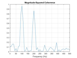
Obtain the magnitude-squared coherence (MSC) for the bivariate time series. The magnitude-squared coherence enables you to identify significant frequency-domain correlation between the two time series. Phase estimates in the cross spectrum are only useful where significant frequency-domain correlation exists.

To prevent obtaining a magnitude-squared coherence estimate, which is identically 1 for all frequencies, you must use an averaged MSC estimator. Both Welch's overlapped segment averaging (WOSA) and mulitaper techniques are appropriate. mscohere implements a WOSA estimator.

Set the window length to 100 samples. This window length contains 10 periods of the 100 Hz sine wave and 20 periods of the 200 Hz sine wave. Use an overlap of 80 samples with the default Hamming window. Input the sample rate explicitly to get the output frequencies in Hz. Plot the magnitude-squared coherence.

[Pxy, F] = mscohere(x, y, hamming(100), 80, 100, Fs); plot(F, Pxy) title('Magnitude-Squared Coherence') xlabel('Frequency (Hz)') grid

You see that the magnitude-squared coherence is greater than 0.8 at 100 and 200 Hz.

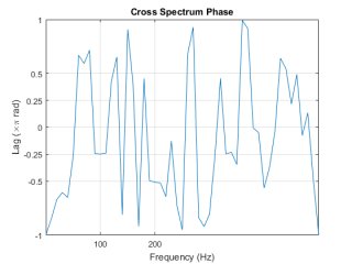
Obtain the cross spectrum of x and y using cpsd. Use the same parameters to obtain the cross spectrum that you used in the MSC estimate. Plot the phase of the cross spectrum and indicate the frequencies with significant coherence between the two times. Mark the known phase lags between the sinusoidal components.

[Cxy, F] = cpsd(x, y, hamming(100), 80, 100, Fs); plot(F, -angle(Cxy)/pi) title('Cross Spectrum Phase') xlabel('Frequency (Hz)') ylabel('Lag (\times\pi rad)') ax = gca; ax.XTick = [100 200]; ax.YTick = [-1 -1/2 -1/4 0 1/4 1/2 1]; grid

You see that, at 100 Hz and 200 Hz, the phase lags estimated from the cross spectrum are close to the true values.

In this example, the cross spectrum estimates are spaced at Hz. You can return the phase estimates at those frequency bins. Keep in mind that the first frequency bin corresponds to 0 Hz, or DC.

phi100 = -angle(Cxy(11)); phi200 = -angle(Cxy(21));